
Deep Learning Hello World In Keras Part2
Assignment 1-b: Deep Learning Hello World! (3-layer MLP)
Objective: To be able to improve upon the basic MLP in part 1 by adding more layers for MNIST Classification
Step 1: Taking care of the imports which includes numpy, datasets, models, layers, optimizers, and utils.
You will also be able to tell if your set-up is correct/complete.
from __future__ import print_function
import numpy as np
from keras.datasets import mnist
from keras.models import Sequential
from keras.models import model_from_json
from keras.layers.core import Dense, Activation
from keras.optimizers import SGD
from keras.utils import np_utils

from matplotlib import pyplot as plt
%matplotlib inline
Step 2: Set-up some constants to be utilized in the training/testing of the model <br> Note: the number of epochs (NB_EPOCH) is reduced to 20
NB_EPOCH = 20
BATCH_SIZE = 128
VERBOSE = 1
NB_CLASSES = 10   # number of outputs = number of digits, i.e. 0,1,2,3,4,5,6,7,8,9
OPTIMIZER = SGD() # Stocastic Gradient Descent optimizer
N_HIDDEN = 128
VALIDATION_SPLIT=0.2 # how much TRAIN dataset is reserved for VALIDATION

np.random.seed(1983)  # for reproducibility
Step 3: Load the MNIST Dataset which are shuffled and split between train and test sets <br>
- X_train is 60000 rows of 28x28 values
- X_test is 10000 rows of 28x28 values
(X_train, y_train), (X_test, y_test) = mnist.load_data()
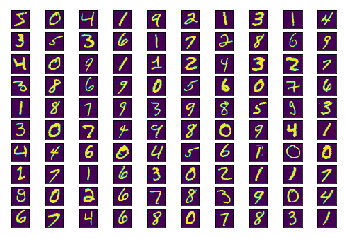
print("First 100 train images:")
for k in range(100):
plt.subplot(10, 10, k+1)
plt.gca().axes.get_yaxis().set_visible(False)
plt.gca().axes.get_xaxis().set_visible(False)
plt.imshow(X_train[k])
First 100 train images:
Step 4: Preprocess the input data by reshaping it, converting it to float, and normalizing it [0-1].
# reshape
X_train = X_train.reshape(60000, 784)
X_test = X_test.reshape(10000, 784)
X_train = X_train.astype('float32')
X_test = X_test.astype('float32')

# normalize
X_train /= 255
X_test /= 255

print(X_train.shape, 'train samples')
print(X_test.shape, 'test samples')
(60000, 784) train samples
(10000, 784) test samples
Step 5: Convert class vectors to binary class matrices; One-Hot-Encoding (OHE)
Y_train = np_utils.to_categorical(y_train, NB_CLASSES)
Y_test = np_utils.to_categorical(y_test, NB_CLASSES)
Step 6: Create the model with 3 layers: Input:784 ==> Hidden:128 ==> Hidden:128 ==> Output:10 (with Softmax activation)
model = Sequential()
model.add(Dense(N_HIDDEN, input_shape=(784,)))
model.add(Activation('relu'))
model.add(Dense(N_HIDDEN))
model.add(Activation('relu'))
model.add(Dense(NB_CLASSES))
model.add(Activation('softmax'))
model.summary()
_________________________________________________________________
Layer (type)                 Output Shape              Param #
=================================================================
dense_1 (Dense)              (None, 128)               100480
_________________________________________________________________
activation_1 (Activation)    (None, 128)               0
_________________________________________________________________
dense_2 (Dense)              (None, 128)               16512
_________________________________________________________________
activation_2 (Activation)    (None, 128)               0
_________________________________________________________________
dense_3 (Dense)              (None, 10)                1290
_________________________________________________________________
activation_3 (Activation)    (None, 10)                0
=================================================================
Total params: 118,282
Trainable params: 118,282
Non-trainable params: 0
_________________________________________________________________
Step 7: Compile the model with categorical_crossentropy loss function, SGD optimizer, and accuracy metric
model.compile(loss='categorical_crossentropy',
              optimizer=OPTIMIZER,
              metrics=['accuracy'])
Step 8: Perform the training with 128 batch size, 200 epochs, and 20 % of the train data used for validation
history = model.fit(X_train, Y_train,
                    batch_size=BATCH_SIZE, epochs=NB_EPOCH,
                    verbose=VERBOSE, validation_split=VALIDATION_SPLIT)
Train on 48000 samples, validate on 12000 samples
Epoch 1/20
48000/48000 [==============================] - 6s - loss: 1.4286 - acc: 0.6594 - val_loss: 0.7242 - val_acc: 0.8373
Epoch 2/20
48000/48000 [==============================] - 2s - loss: 0.5890 - acc: 0.8547 - val_loss: 0.4472 - val_acc: 0.8845
Epoch 3/20
48000/48000 [==============================] - 2s - loss: 0.4366 - acc: 0.8833 - val_loss: 0.3698 - val_acc: 0.8998
Epoch 4/20
48000/48000 [==============================] - 2s - loss: 0.3782 - acc: 0.8947 - val_loss: 0.3317 - val_acc: 0.9073
Epoch 5/20
48000/48000 [==============================] - 3s - loss: 0.3455 - acc: 0.9022 - val_loss: 0.3088 - val_acc: 0.9128
Epoch 6/20
48000/48000 [==============================] - 3s - loss: 0.3228 - acc: 0.9078 - val_loss: 0.2929 - val_acc: 0.9167
Epoch 7/20
48000/48000 [==============================] - 2s - loss: 0.3054 - acc: 0.9124 - val_loss: 0.2803 - val_acc: 0.9194
Epoch 8/20
48000/48000 [==============================] - 3s - loss: 0.2914 - acc: 0.9161 - val_loss: 0.2689 - val_acc: 0.9229
Epoch 9/20
48000/48000 [==============================] - 2s - loss: 0.2790 - acc: 0.9196 - val_loss: 0.2601 - val_acc: 0.9243
Epoch 10/20
48000/48000 [==============================] - 2s - loss: 0.2679 - acc: 0.9228 - val_loss: 0.2511 - val_acc: 0.9266
Epoch 11/20
48000/48000 [==============================] - 2s - loss: 0.2581 - acc: 0.9256 - val_loss: 0.2437 - val_acc: 0.9281
Epoch 12/20
48000/48000 [==============================] - 2s - loss: 0.2488 - acc: 0.9282 - val_loss: 0.2364 - val_acc: 0.9307
Epoch 13/20
48000/48000 [==============================] - 3s - loss: 0.2406 - acc: 0.9308 - val_loss: 0.2298 - val_acc: 0.9340
Epoch 14/20
48000/48000 [==============================] - 3s - loss: 0.2332 - acc: 0.9330 - val_loss: 0.2234 - val_acc: 0.9355
Epoch 15/20
48000/48000 [==============================] - 2s - loss: 0.2257 - acc: 0.9351 - val_loss: 0.2174 - val_acc: 0.9378
Epoch 16/20
48000/48000 [==============================] - 2s - loss: 0.2186 - acc: 0.9370 - val_loss: 0.2125 - val_acc: 0.9379
Epoch 17/20
48000/48000 [==============================] - 2s - loss: 0.2123 - acc: 0.9379 - val_loss: 0.2066 - val_acc: 0.9418
Epoch 18/20
48000/48000 [==============================] - 2s - loss: 0.2060 - acc: 0.9403 - val_loss: 0.2013 - val_acc: 0.9427
Epoch 19/20
48000/48000 [==============================] - 2s - loss: 0.2002 - acc: 0.9420 - val_loss: 0.1969 - val_acc: 0.9448
Epoch 20/20
48000/48000 [==============================] - 2s - loss: 0.1945 - acc: 0.9436 - val_loss: 0.1929 - val_acc: 0.9464
Step 9: Evaluate the model on the test dataset (10,000 images)
score = model.evaluate(X_test, Y_test, verbose=VERBOSE)
print("\nTest score:", score[0])
print('Test accuracy:', score[1])
 9088/10000 [==========================>...] - ETA: 0s
Test score: 0.193726402299
Test accuracy: 0.9456
[Optional] Step 10: Save the model (serialized) to JSON
model_json = model.to_json()
with open("model.json", "w") as json_file:
    json_file.write(model_json)
%ls
 Volume in drive C is Windows
 Volume Serial Number is 7252-C405

 Directory of C:\Users\cobalt\workspace

09/17/2017  04:28 PM    <DIR>          .
09/17/2017  04:28 PM    <DIR>          ..
09/17/2017  01:51 PM    <DIR>          .ipynb_checkpoints
01/07/2017  12:22 PM    <DIR>          .metadata
09/17/2017  01:16 PM            50,073 DeepLearningHelloWorld.ipynb
09/17/2017  04:28 PM            83,748 DeepLearningHelloWorldPart2.ipynb
01/08/2017  10:52 AM    <DIR>          Hello
01/08/2017  10:52 AM    <DIR>          Hellocpp11
01/09/2017  04:45 PM    <DIR>          HelloOpenCV
09/17/2017  01:07 PM            42,528 model.h5
09/17/2017  04:30 PM             1,875 model.json
01/07/2017  12:22 PM    <DIR>          RemoteSystemsTempFiles
               4 File(s)        178,224 bytes
               8 Dir(s)  199,338,438,656 bytes free
[Optional] Step 11: Save the model weights
model.save_weights("model.h5")
%ls
 Volume in drive C is Windows
 Volume Serial Number is 7252-C405

 Directory of C:\Users\cobalt\workspace

09/17/2017  04:30 PM    <DIR>          .
09/17/2017  04:30 PM    <DIR>          ..
09/17/2017  01:51 PM    <DIR>          .ipynb_checkpoints
01/07/2017  12:22 PM    <DIR>          .metadata
09/17/2017  01:16 PM            50,073 DeepLearningHelloWorld.ipynb
09/17/2017  04:30 PM            56,494 DeepLearningHelloWorldPart2.ipynb
01/08/2017  10:52 AM    <DIR>          Hello
01/08/2017  10:52 AM    <DIR>          Hellocpp11
01/09/2017  04:45 PM    <DIR>          HelloOpenCV
09/17/2017  04:31 PM           490,640 model.h5
09/17/2017  04:30 PM             1,875 model.json
01/07/2017  12:22 PM    <DIR>          RemoteSystemsTempFiles
               4 File(s)        599,082 bytes
               8 Dir(s)  199,338,012,672 bytes free
[Optional] Step 12: Load the saved model
json_file = open('model.json', 'r')
loaded_model_json = json_file.read()
json_file.close()
loaded_model = model_from_json(loaded_model_json)
loaded_model.load_weights("model.h5")
[Optional] Step 13: Compile and evaluate loaded model
loaded_model.compile(loss='categorical_crossentropy',
              optimizer=OPTIMIZER,
              metrics=['accuracy'])
score = loaded_model.evaluate(X_test, Y_test, verbose=VERBOSE)
print("\nTest score:", score[0])
print('Test accuracy:', score[1])
 9600/10000 [===========================>..] - ETA: 0s
Test score: 0.193726402299
Test accuracy: 0.9456
- mkc