
Basic Feature Detection
“The fact that objects in the world appear in different ways depending on the scale of observation has important implications if one aims at describing them. It shows that the notion of scale is of utmost importance when processing unknown measurement data by automatic methods.”
Tony Lindeberg
Feature detection is an essential component of many computer vision applications.
Edge detection
%matplotlib inline
import matplotlib.pyplot as plt
import numpy as np
plt.rcParams['image.cmap'] = 'gray'
plt.rcParams['image.interpolation'] = 'none'
import skdemo
from skimage import data
# Rename module so we don't shadow the builtin function
import skimage.filters as filters
image = data.camera()
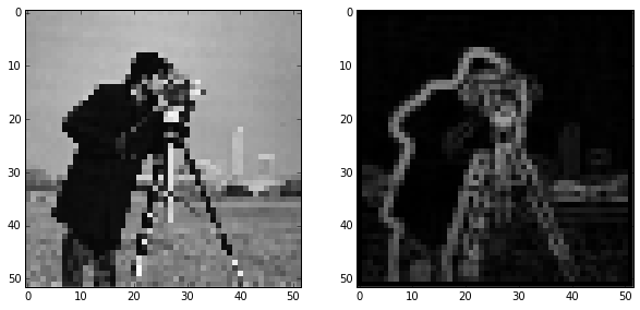
pixelated = image[::10, ::10]
gradient = filters.sobel(pixelated)
skdemo.imshow_all(pixelated, gradient)
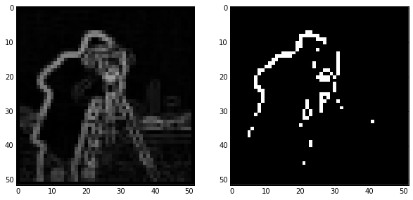
skdemo.imshow_all(gradient, gradient > 0.4)
Canny edge detector
The Canny edge detector combines the Sobel filter with a few other steps to give a binary edge image. The steps are as follows:
- Gaussian filter
- Sobel filter
- Non-maximal suppression
- Hysteresis thresholding
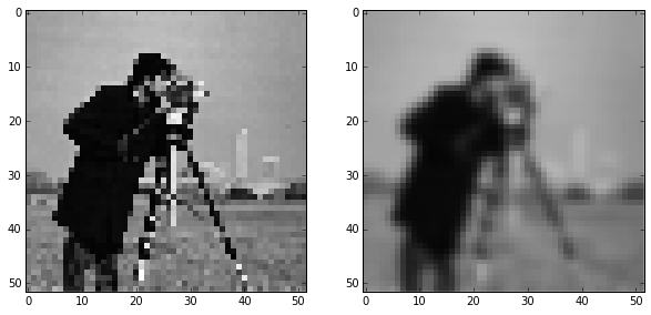
Step 1: Gaussian filter
from skimage import img_as_float

sigma = 1  # Standard-deviation of Gaussian; larger smooths more.
pixelated_float = img_as_float(pixelated)
pixelated_float = pixelated
smooth = filters.gaussian_filter(pixelated_float, sigma)
skdemo.imshow_all(pixelated_float, smooth)
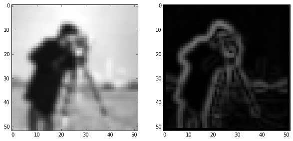
Step 2: Sobel filter
gradient_magnitude = filters.sobel(smooth)
skdemo.imshow_all(smooth, gradient_magnitude)
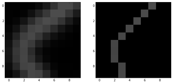
Step 3: Non-maximal suppression
zoomed_grad = gradient_magnitude[15:25, 5:15]
maximal_mask = np.zeros_like(zoomed_grad)
# This mask is made up for demo purposes
maximal_mask[range(10), (7, 6, 5, 4, 3, 2, 2, 2, 3, 3)] = 1
grad_along_edge = maximal_mask * zoomed_grad
skdemo.imshow_all(zoomed_grad, grad_along_edge, limits='dtype')
Step 4: Hysteresis thresholding
from skimage import color

low_threshold = 0.2
high_threshold = 0.3
label_image = np.zeros_like(pixelated)
# This uses `gradient_magnitude` which has NOT gone through non-maximal-suppression.
label_image[gradient_magnitude > low_threshold] = 1
label_image[gradient_magnitude > high_threshold] = 2
demo_image = color.label2rgb(label_image, gradient_magnitude,
                             bg_label=0, colors=('yellow', 'red'))
plt.imshow(demo_image);
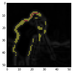
The red points here are above high_threshold and are seed points for edges. The yellow points are edges if connected (possibly by other yellow points) to seed points; i.e. isolated groups of yellow points will not be detected as edges.
Note that the demo above is on the edge image before non-maximal suppression, but in reality, this would be done on the image after non-maximal suppression. There isn’t currently an easy way to get at the intermediate result.
The Canny edge detector
from IPython.html import widgets
from skimage import data
from skimage import feature

image = data.coins()

def canny_demo(**kwargs):
    edges = feature.canny(image, **kwargs)
    plt.imshow(edges)
    plt.show()
# As written, the following doesn't actually interact with the
# `canny_demo` function. Figure out what you need to add.
widgets.interact(canny_demo);  # <-- add keyword arguments for `canny`
<function __main__.canny_demo>
Hough transforms
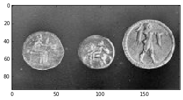
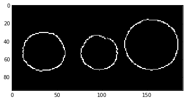
Circle detection
image = data.coins()[0:95, 180:370]
plt.imshow(image);
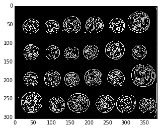
edges = feature.canny(image, sigma=3, low_threshold=10, high_threshold=60)
plt.imshow(edges);
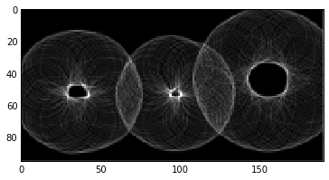
from skimage.transform import hough_circle

hough_radii = np.arange(15, 30, 2)
hough_response = hough_circle(edges, hough_radii)
print(edges.shape)
print(hough_response.shape)

(95, 190)
(8, 95, 190)


# Use max value to intelligently rescale the data for plotting.
h_max = hough_response.max()

def hough_responses_demo(i):
    # Use `plt.title` to add a meaningful title for each index.
    plt.imshow(hough_response[i, :, :], vmax=h_max*0.5)
    plt.show()
widgets.interact(hough_responses_demo, i=(0, len(hough_response)-1));
Reference:
 [1] https://github.com/scikit-image/scikit-image
 [2] Richard Szeliski. Computer Vision: Algorithms and Applications. Springer, New York, 2010.
<iframe src=”http://mesh.brown.edu/engn1610/szeliski/04-featuredetectionandmatching.pdf” width=100% height=”888”></iframe>