excerpts from opencv3 blueprints

Factors that affect object detection

Data collection

This step includes collecting the necessary data for building and testing your object detector. The data can be acquired from a range of sources going from video sequences to images captured by a webcam. This step will also make sure that the data is formatted correctly to be ready to be passed to the training stage.

An example of positive and negative training data for an object model:

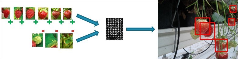
• Positive - contains the different presentations of the object you want to detect (this means object instances under different lighting conditions, different scales, different orientations, small shape changes, and so on).

For the positive samples, only use natural occurring samples. There are many tools out there that create artificially rotated, translated, and skewed images to turn a small training set into a large training set. However, research has proven that the resulting detector is less performant than simply collecting positive object samples that cover the actual situation of your application. Better use a small set of decent high quality object samples, rather than using a large set of low quality non-representative samples for your case.

• Negatives - contains everything that you do not want to detect with your model. For the negative samples, there are two possible approaches, but both start from the principle that you collect negative samples in the situation where your detector will be used, which is very different from the normal way of training object detects, where just a large set of random samples not containing the object are being used as negatives.

Either point a camera at your scene and start grabbing random frames to sample negative windows from.

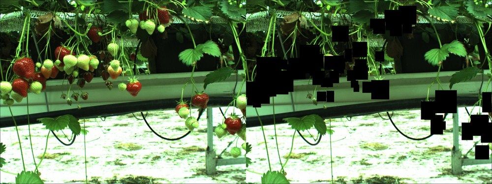
Or use your positive images to your advantage. Cut out the actual object regions and make the pixels black. Use those masked images as negative training data. Keep in mind that in this case the ratio between background information and actual object occurring in the window needs to be large enough. If your images are filled with object instances, cutting them will result in a complete loss of relevant background information and thus reduce the discriminative power of your negative training set.

Efficiently collecting data in this way ensures that you will end up with a very robust model for your specific application! However, keep in mind that this also has some consequences. The resulting model will not be robust towards different situations than the ones trained for. However, the benefit in training time and the reduced need of training samples completely outweighs this downside.

Note

Software for negative sample generation based on OpenCV 3 can be found at https://github.com/OpenCVBlueprints/OpenCVBlueprints/tree/master/chapter_5/source_code/generate_negatives/.

You can use the negative sample generation software to generate samples like you can see in the following figure, where object annotations of strawberries are removed and replaced by black pixels.

Creating object annotation files for the positive samples

When preparing your positive data samples, it is important to put some time in your annotations, which are the actual locations of your object instances inside the larger images. Without decent annotations, you will never be able to create decent object detectors.

Software for object annotation based on OpenCV 3 can be found at https://github.com/OpenCVBlueprints/OpenCVBlueprints/tree/master/chapter_5/source_code/object_annotation/.

The OpenCV team was kind enough to also integrate this tool into the main repository under the apps section. This means that if you build and install the OpenCV apps during installation, that the tool is also accessible by using the following command:

/opencv_annotation -images -annotations

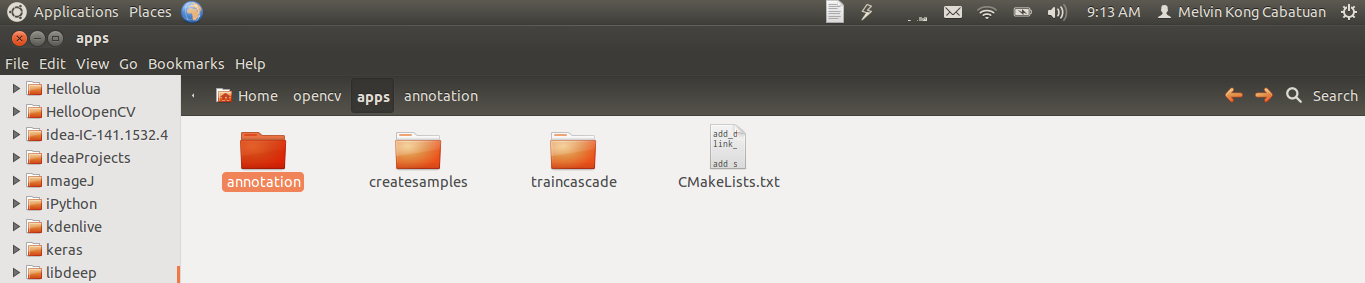
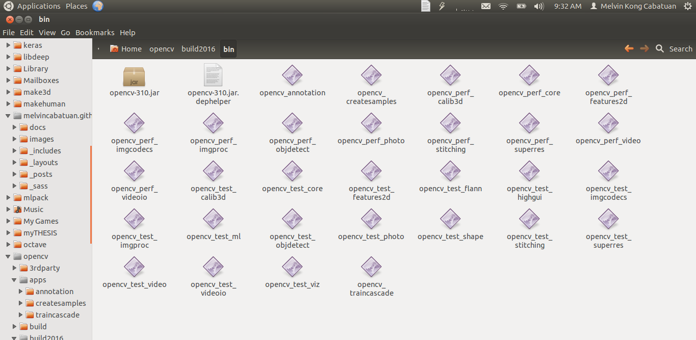
Sample executables after OpenCV 3.0 install: (Notice: opencv_annotation, opencv_createsamples, and opencv_traincascade)

Parsing your positive dataset into the OpenCV data vector

The sample creation tool can be found at https://github.com/Itseez/opencv/tree/master/apps/createsamples/ and should be built automatically if OpenCV was installed correctly, which makes it usable through the opencv_createsamples command.

reating the sample vector is quite easy and straightforward by applying the following instruction from the command line interface:

./opencv_createsamples –info annotations.txt –vec images.vec –bg negatives.txt –num amountSamples –w model_width –h model_height

info: Add here the annotation file that was created using the object annotation software. Make sure that the format is correct, that there is no empty line at the bottom of the file and that the coordinates fall inside the complete image region. This annotation file should only contain positive image samples and no negative image samples as some online tutorials suggest. This would train your model to recognize negative samples as positives, which is not what we desire.

vec: This is the data format OpenCV will use to store all the image information and is the file that you created using the create samples software provided by OpenCV itself.

num: This is the actual number of annotations that you have inside the vector file over all the images presented to the algorithm. If you have no idea anymore how many objects you have actually annotated, then run the annotation counter software supplied.

The sample counting tool can be found at https://github.com/OpenCVBlueprints/OpenCVBlueprints/tree/master/chapter_5/source_code/count_samples/ and can be executed by the following command:

./count_samples -file <annotations.txt>

w and h: These are the two parameters that specify the final model dimensions. Keep in mind that these dimensions will immediately define the smallest object that you will be able to detect. Keep the size of the actual model therefore smaller than the smallest object you want to detect in your test images. Take, for example, the Viola and Jones face detector, which was trained on samples of 24x24 pixels, and will never be able to detect faces of 20x20 pixels.

If you have created a working classifier with, for example, 24x24 pixel dimensions and you still want to detect smaller objects, then a solution could be to upscale your images before applying the detector. However, keep in mind that if your actual object is, for example, 10x10 pixels, then upscaling that much will introduce tons of artifacts, which will render your model detection capabilities useless.

A last point of attention is how you can decide which is an effective model size for your purpose. On the one hand, you do not want it to be too large so that you can detect small object instances, on the other hand, you want enough pixel information so that separable features can be found.

You can find a small code snippet that can help you out with defining these ideal model dimensions based on the average annotation dimensions at the following location:

https://github.com/OpenCVBlueprints/OpenCVBlueprints/tree/master/chapter_5/source_code/average_dimensions/.

Basically, what this software does is it takes an annotation file and processes the dimensions of all your object annotations. It then returns an average width and height of your object instances. You then need to apply a scaling factor to assign the dimensions of the smallest detectable object.

For example:

• Take a set of annotated apples in an orchard. You got a set of annotated apple tree images of which the annotations are stored in the apple annotation file.

• Pass the apple annotation file to the software snippet which returns you the average apple width and apple height. For now, we suppose that the dimensions for [w_average h_average] are [60 60].

• If we would use those [60 60] dimensions, then we would have a model that can only detect apples equal and larger to that size. However, moving away from the tree will result in not a single apple being detected anymore, since the apples will become smaller in size.

Therefore, I suggest reducing the dimensions of the model to, for example, [30 30]. This will result in a model that still has enough pixel information to be robust enough and it will be able to detect up to half the apples of the training apples size.

Generally speaking, the rule of thumb can be to take half the size of the average dimensions of the annotated data and ensure that your largest dimension is not bigger than 100 pixels. This last guideline is to ensure that training your model will not increase exponentially in time due to the large model size. If your largest dimension is still over 100 pixels, then just keep halving the dimensions until you go below this threshold.

Model Training

In this step, you will use the data gathered in the first step to train an object model that will be able to detect that model class. Here, the different training parameters will be investigated and the focus will be on defining the correct settings for the application.

• Parameter selection when training an object model

The training itself is based on applying the boosting algorithm on either Haar wavelet features or Local Binary Pattern features.

If you are interested in knowing all the technical details of the feature calculation, then have a look at the following papers which describe them in detail:

*HAAR*: Papageorgiou, Oren and Poggio, "A general framework for object detection", International Conference on Computer Vision, 1998.

*LBP*: T. Ojala, M. Pietikäinen, and D. Harwood (1994), "Performance evaluation of texture measures with classification based on Kullback discrimination of distributions", Proceedings of the 12th IAPR International Conference on Pattern Recognition (ICPR 1994), vol. 1, pp. 582 - 585.

Testing and Validation

Once you have a trained object model, you can use it to try and detect object instances in the given test images. Compare each detection with a manually defined ground truth of the test data.

Ground truth means a set of measurements that is known to be much more accurate than measurements from the system you are testing, e.x. manually annotated, problem-specific labels in computer vision.

A good and accurately annotated ground truth set will always give you a more reliable object model and will yield better test and accuracy results.

Make sure that the bounding box contains the complete object, but at the same time avoid as much background information as possible. The ratio of object information compared to background information should always be larger than 80%. Otherwise, the background could yield enough features to train your model on and the end result will be your detector model focusing on the wrong image information.

Viola and Jones suggests using squared annotations, based on a 24x24 pixel model, because it fits the shape of a face. However, this is not mandatory! If your object class is more rectangular like, then do annotate rectangular bounding boxes instead of squares. It is observed that people tend to push rectangular shaped objects in a square model size, and then wonder why it is not working correctly. Take, for example, the case of a pencil detector, where the model dimensions will be more like 10x70 pixels, which is in relation to the actual pencil dimensions.

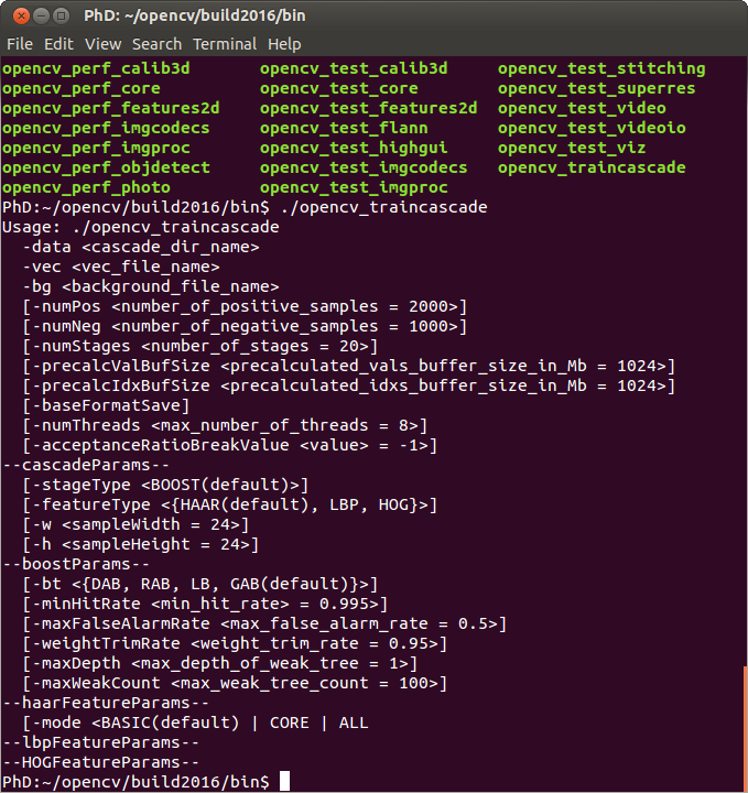
The cascade classification training tool can be found at https://github.com/Itseez/opencv/tree/master/apps/traincascade/. If you build the OpenCV apps and installed them, then it will be directly accessible by executing the ./train_cascade command.

• data: This parameter contains the folder where you will output your training results. Since the creation of folders is OS specific, OpenCV decided that they will let users handle the creation of the folder. If you do not make it in advance, training results will not be stored correctly. The folder will contain a set of XML files, one for the training parameters, one for each trained stage and finally a combined XML file containing the object model.

• numPos: This is the amount of positive samples that will be used in training each stage of weak classifiers. Keep in mind that this number is not equal to the total amount of positive samples. The classifier training process is able to reject positive samples that are wrongfully classified by a certain stage limiting further stages to use that positive sample. A good guideline in selecting this parameter is to multiply the actual amount of positive samples, retrieved by the sample counter snippet, with a factor of 0.85.

• numNeg: This is the amount of negative samples used at each stage. However, this is not the same as the amount of negative images that were supplied by the negative data. The training samples negative windows from these images in a sequential order at the model size dimensions. Choosing the right amount of negatives is highly dependent on your application.

  If your application has close to no variation, then supplying a small number of windows could simply do the trick because they will contain most of the background variance. On the other hand, if the background variation is large, a huge number of samples would be needed to ensure that you train as much random background noise as possible into your model. A good start is taking a ratio between the number of positive and the number of negative samples equaling 0.5, so double the amount of negative versus positive windows.

Keep in mind that each negative window that is classified correctly at an early stage will be discarded for training in the next stage since it cannot add any extra value to the training process. Therefore, you must be sure that enough unique windows can be grabbed from the negative images. For example, if a model uses 500 negatives at each stage and 100% of those negatives get correctly classified at each stage, then training a model of 20 stages will need 10,000 unique negative samples! Considering that the sequential grabbing of samples does not ensure uniqueness, due to the limited pixel wise movement, this amount can grow drastically.

• numStages: This is the amount of weak classifier stages, which is highly dependent on the complexity of the application.

  The more stages, the longer the training process will take since it becomes harder at each stage to find enough training windows and to find features that correctly separate the data. Moreover, the training time increases in an exponential manner when adding stages.

  Therefore, I suggest looking at the reported acceptance ratio that is outputted at each training stage. Once this reaches values of 10^(-5), you can conclude that your model will have reached the best descriptive and generalizing power it could get, according to the training data provided.

  Avoid training it to levels of 10^(-5) or lower to avoid overtraining your cascade on your training data. Of course, depending on the amount of training data supplied, the amount of stages to reach this level can differ a lot.

• bg: This refers to the location of the text file that contains the locations of the negative training images, also called the negative samples description file.

• vec: This refers to the location of the training data vector that was generated in the previous step using the create_samples application, which is built-in to the OpenCV 3 software.

• precalcValBufSize and precalcIdxBufSize: These parameters assign the amount of memory used to calculate all features and the corresponding weak classifiers from the training data. If you have enough RAM memory available, increase these values to 2048 MB or 4096 MB, which will speed up the precalculation time for the features drastically.

• featureType: Here, you can choose which kind of features are used for creating the weak classifiers.

  HAAR wavelets are reported to give higher accuracy models.
  However, consider training test classifiers with the LBP parameter. It decreases training time of an equal sized model drastically due to the integer calculations instead of the floating point calculations.

• minHitRate: This is the threshold that defines how much of your positive samples can be misclassified as negatives at each stage. The default value is 0.995, which is already quite high. The training algorithm will select its stage threshold so that this value can be reached.

  Making it 0.999, as many people do, is simply impossible and will make your training stop probably after the first stage. It means that only 1 out of 1,000 samples can be wrongly classified over a complete stage. If you have very challenging data, then lowering this, for example, to 0.990 could be a good start to ensure that the training actually ends up with a useful model.

• maxFalseAlarmRate: This is the threshold that defines how much of your negative samples need to be classified as negatives before the boosting process should stop adding weak classifiers to the current stage. The default value is 0.5 and ensures that a stage of weak classifier will only do slightly better than random guessing on the negative samples. Increasing this value too much could lead to a single stage that already filters out most of your given windows, resulting in a very slow model at detection time due to the vast amount of features that need to be validated for each window. This will simply remove the large advantage of the concept of early window rejection.

The parameters discussed earlier are the most important ones to dig into when trying to train a successful classifier. Once this works, you can increase the performance of your classifier even more, by looking at the way boosting forms its weak classifiers. This can be adapted by the -maxDepth and -maxWeakCount parameters. However, for most cases, using stump weak classifiers (single layer decision trees) on single features is the best way to start, ensuring that single stage evaluation is not too complex and thus fast at detection time.

“If you have a positive attitude and constantly strive to give your best effort, eventually you will overcome your immediate problems and find you are ready for greater challenges.”
Pat Riley