SCIKIT's Image Segmentation

“Research is to see what everybody else has seen, and to think what nobody else has thought.”
Albert Szent-Gyorgyi

import numpy as np
%matplotlib inline
from matplotlib import pyplot as plt


import skdemo
plt.rcParams['image.cmap'] = 'spectral'
from skimage import io, segmentation as seg, color

url = '../images/spice_1.jpg'
image = io.imread(url)


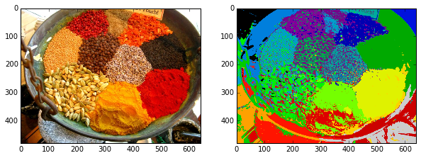
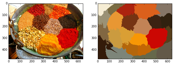
labels = seg.slic(image, n_segments=18, compactness=10)
skdemo.imshow_all(image, labels.astype(float) / labels.max())
print(labels)

[[ 0  0  0 ...,  4  4  4]
 [ 0  0  0 ...,  4  4  4]
 [ 0  0  0 ...,  4  4  4]
 ..., 
 [15 15 15 ..., 19 19 19]
 [15 15 15 ..., 19 19 19]
 [15 15 15 ..., 19 19 19]]

_config.yml

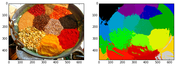
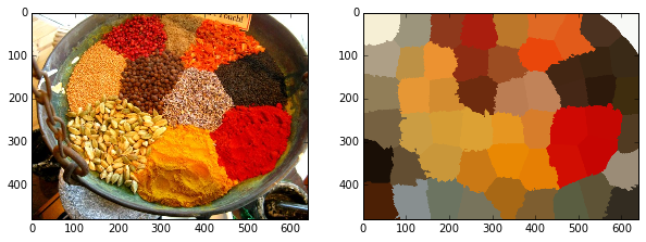
labels = seg.slic(image, n_segments=18, compactness=40)
skdemo.imshow_all(image, labels.astype(float) / labels.max())
print(labels)

[[ 0  0  0 ...,  4  4  4]
 [ 0  0  0 ...,  4  4  4]
 [ 0  0  0 ...,  4  4  4]
 ..., 
 [15 15 15 ..., 19 19 19]
 [15 15 15 ..., 19 19 19]
 [15 15 15 ..., 19 19 19]]

_config.yml

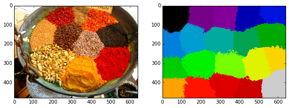
labels = seg.slic(image, n_segments=18, compactness=100)
skdemo.imshow_all(image, labels.astype(float) / labels.max())
print(labels)

[[ 0  0  0 ...,  4  4  4]
 [ 0  0  0 ...,  4  4  4]
 [ 0  0  0 ...,  4  4  4]
 ..., 
 [15 15 15 ..., 19 19 19]
 [15 15 15 ..., 19 19 19]
 [15 15 15 ..., 19 19 19]]

_config.yml

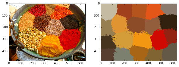
def mean_color(image, labels):
    out = np.zeros_like(image)
    for label in np.unique(labels):
        indices = np.nonzero(labels == label)
        out[indices] = np.mean(image[indices], axis=0)
    return out

skdemo.imshow_all(image, mean_color(image, labels))

_config.yml

labels = seg.slic(image, n_segments=24, compactness=40,
                  sigma=2, enforce_connectivity=True)
label_image = mean_color(image, labels)
skdemo.imshow_all(image, label_image)

_config.yml

def myfunc(*args, **kwargs):
    labels = seg.slic(image, *args, **kwargs)
    color = mean_color(image, labels) 
    skdemo.imshow_all(image, color)
    
from IPython.html import widgets
w = widgets.interactive(myfunc, compactness = (5, 200, 10), n_segments =(25, 200, 15), enforce_connectivity = True)
w.msg_throttle = 1
w

_config.yml

def myfunc(*args, **kwargs):
    labels = seg.slic(image, *args, **kwargs)
    color = mean_color(image, labels) 
    skdemo.imshow_all(image, color)
    
from IPython.html import widgets
w = widgets.interactive(myfunc, compactness = (5, 100, 5), n_segments =(25, 200, 15), sigma = (0.,5.,0.1), enforce_connectivity = True)
w.msg_throttle = 1
w

_config.yml

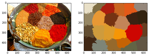
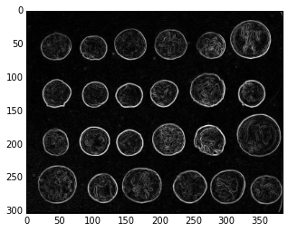
Image types: boundary images

Often, the contrast between regions is not sufficient to distinguish them, but there is a clear boundary between the two. Using an edge detector on these images, followed by a watershed, often gives very good segmentation.

from skimage import data, filters as filters
from matplotlib import pyplot as plt, cm

coins = data.coins()
edges = filters.sobel(coins)

plt.imshow(edges, cmap='gray');

_config.yml

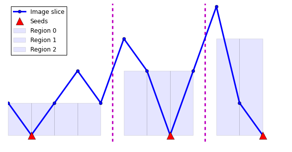
The watershed algorithm finds the regions between these edges. It does so by envisioning the pixel intensity as height on a topographic map. It then “floods” the map from the bottom up, starting from seed points. These flood areas are called “watershed basins” and when they meet, they form the image segmentation.

from skimage.morphology import watershed
from scipy import ndimage as nd

x = np.array([0, 1, 2, 3, 4, 5, 6, 7, 8, 9, 10, 11])
y = np.array([1, 0, 1, 2, 1, 3, 2, 0, 2, 4, 1, 0])

seeds = nd.label(y == 0)[0]
seed_positions = np.argwhere(seeds)[:, 0]

print("Seeds:", seeds)
print("Seed positions:", seed_positions)

# ------------------------------- #
result = watershed(y, seeds)
# ------------------------------- #

# You can ignore the code below--it's just
# to make a pretty plot of the results.
plt.figure(figsize=(10, 5))
plt.plot(y, '-o', label='Image slice', linewidth=3)
plt.plot(seed_positions, np.zeros_like(seed_positions), 'r^',
         label='Seeds', markersize=15)

for n, label in enumerate(np.unique(result)):
    mask = (result == label)
    plt.bar(x[mask][:-1], result[mask][:-1],
            width=1, label='Region %d' % n,
            alpha=0.1)

plt.vlines(np.argwhere(np.diff(result)) + 0.5, -0.2, 4.1, 'm',
           linewidth=3, linestyle='--')

plt.legend(loc='upper left', numpoints=1)
plt.axis('off')
plt.ylim(-0.2, 4.1);

Seeds: [0 1 0 0 0 0 0 2 0 0 0 3]
Seed positions: [ 1  7 11]

_config.yml

from scipy import ndimage as nd
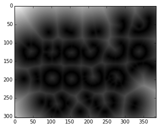
threshold = 0.4

# Euclidean distance transform
# How far do we have to travel from a non-edge to find an edge?
non_edges = (edges < threshold)
distance_from_edge = nd.distance_transform_edt(non_edges)

plt.imshow(distance_from_edge, cmap='gray');

_config.yml

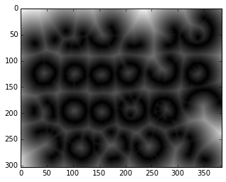
threshold = 0.35

# Euclidean distance transform
# How far do we have to travel from a non-edge to find an edge?
non_edges = (edges < threshold)
distance_from_edge = nd.distance_transform_edt(non_edges)

plt.imshow(distance_from_edge, cmap='gray');

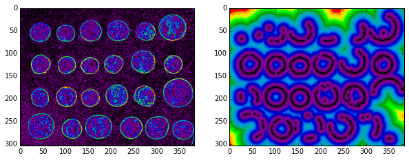
skdemo.imshow_all(edges/edges.max(), distance_from_edge/distance_from_edge.max());

_config.yml

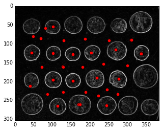
from skimage import feature

# -------------------------------------------------#
peaks = feature.peak_local_max(distance_from_edge)
print("Peaks shape:", peaks.shape)
# -------------------------------------------------#

peaks_image = np.zeros(coins.shape, np.bool)
peaks_image[tuple(np.transpose(peaks))] = True
seeds, num_seeds = nd.label(peaks_image)

plt.imshow(edges, cmap='gray')
plt.plot(peaks[:, 1], peaks[:, 0], 'ro');
plt.axis('image')

Peaks shape: (40, 2)





(-0.5, 383.5, 302.5, -0.5)

_config.yml

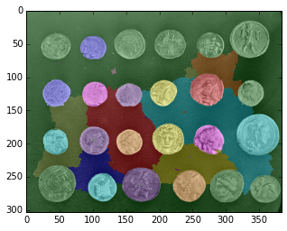
ws = watershed(edges, seeds)

from skimage import color
plt.imshow(color.label2rgb(ws, coins));

_config.yml

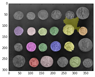
from skimage.measure import regionprops

regions = regionprops(ws)

ws_updated = ws.copy()
for region in regions:
    if region.eccentricity > 0.6:
        ws_updated[ws_updated == region.label] = 0

plt.imshow(color.label2rgb(ws_updated, coins, bg_label=0));

_config.yml

Written on April 6, 2015