
When Straight Is Not Enough
import numpy as np
import pandas as pd
import matplotlib.pyplot as plt
plt.style.use('seaborn')
# Data: https://data.worldbank.org/country/philippines
raw = pd.read_excel("API_PHL_DS2_en_excel_v2_716225.xls", header=3, sheet_name='Data')
raw.set_index('Indicator Name', inplace=True)
# Choose Numeric Values ONLY
data = raw.iloc[:,3:]
data = data.T
# Basic plotting
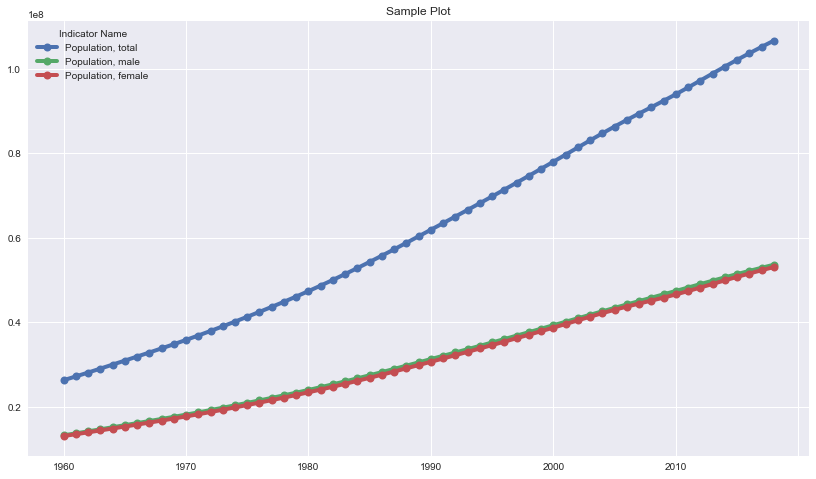
indicators = ['Population, total','Population, male','Population, female']
data[indicators].plot(grid=True, figsize=(14,8), title="Sample Plot", lw = 4, marker='.', markersize=16);
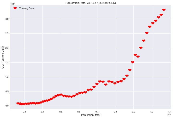
Population, total vs. GDP (current US $)
fig, ax = plt.subplots(figsize=(12,8));
plt.grid('on')
ax.scatter(data['Population, total'], data['GDP (current US$)'], label='Training Data', marker='$❤$', s = 200, c = 'r');
ax.legend()
ax.set_xlabel('Population, total')
ax.set_ylabel('GDP (current US$)')
ax.set_title('Population, total vs. GDP (current US$)')
Text(0.5, 1.0, 'Population, total vs. GDP (current US$)')
from sklearn import linear_model

X = data['Population, total'].values[:-1]
y = data['GDP (current US$)'].values[:-1]

X = X.reshape(-1, 1)

mymodel = linear_model.LinearRegression().fit(X, y)

print("slope =", mymodel.coef_)
print("intercept =", mymodel.intercept_)
slope = [3366.65440331]
intercept = -129367421881.78075
# Predicted
x = np.linspace(data['Population, total'].min(), data['Population, total'].max(), 100)
y = mymodel.predict(x.reshape(-1, 1)).flatten()

fig, ax = plt.subplots(figsize=(12,8));
ax.plot(x, y, 'bo-', label='Prediction: $3366.65x - 129367421881$')
ax.scatter(data['Population, total'], data['GDP (current US$)'], label='Training Data', marker='$❤$', s = 200, c = 'r');
ax.set_xlabel('Population, total')
ax.set_ylabel('GDP (current US$)')
ax.set_title('Population, total vs. GDP (current US$)')
ax.legend()
plt.grid('on')
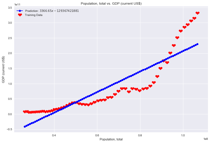
Sometime straight is not the best model
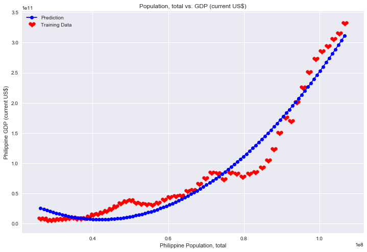
# BONUS ANSWER: Polynomial Fitting

from sklearn.preprocessing import PolynomialFeatures
from sklearn.linear_model import LinearRegression

X = data['Population, total'].values[:-1] # get rid of nan value
y = data['GDP (current US$)'].values[:-1]

# preprocess
X    = X.reshape(-1, 1)
poly = PolynomialFeatures(degree = 2)
X    = poly.fit_transform(X)

mymodel2 = linear_model.LinearRegression()
mymodel2.fit(X, y)

print("slope =", mymodel2.coef_)
print("intercept =", mymodel2.intercept_)
slope = [ 0.00000000e+00 -6.16715871e+03  7.31697259e-05]
intercept = 136991174065.16896
# Predicted
x = np.linspace(data['Population, total'].min(), data['Population, total'].max(), 100)
x = poly.fit_transform(x.reshape(-1, 1))
y = mymodel2.predict(x).flatten()

fig, ax = plt.subplots(figsize=(12,8));
ax.plot(x[:,1], y, 'bo-', label='Prediction')
ax.scatter(data['Population, total'], data['GDP (current US$)'], label='Training Data', marker='$❤$', s = 200, c = 'r');
ax.set_xlabel('Philippine Population, total')
ax.set_ylabel('Philippine GDP (current US$)')
ax.set_title('Population, total vs. GDP (current US$)')
ax.legend()
plt.grid('on')
Written on February 28, 2020