Colour Part 1

“The mind of the painter must resemble a mirror, which always takes the colour of the object it reflects and is completely occupied by the images of as many objects as are in front of it. Therefore you must know, Oh Painter! that you cannot be a good one if you are not the universal master of representing by your art every kind of form produced by nature. And this you will not know how to do if you do not see them, and retain them in your mind.”
Leonardo Da Vinci

from skimage import data

image = data.camera()


%matplotlib inline
import matplotlib.pyplot as plt
import numpy as np


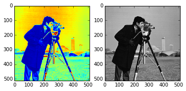
fig, (ax_jet, ax_gray) = plt.subplots(ncols=2)
ax_jet.imshow(image, cmap='jet')
ax_gray.imshow(image, cmap='gray');

_config.yml

<matplotlib.figure.Figure at 0xaf27792c>



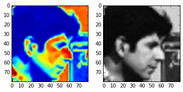
face = image[80:160, 200:280]
fig, (ax_jet, ax_gray) = plt.subplots(ncols=2)
ax_jet.imshow(face, cmap='jet')
ax_gray.imshow(face, cmap='gray');

_config.yml

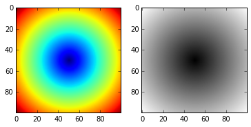
X, Y = np.ogrid[-5:5:0.1, -5:5:0.1]
R = np.sqrt(X**2 + Y**2)

fig, (ax_jet, ax_gray) = plt.subplots(1, 2)
ax_jet.imshow(R, cmap='jet')
ax_gray.imshow(R, cmap='gray');

_config.yml

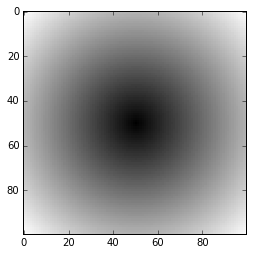
plt.rcParams['image.cmap'] = 'gray'

plt.rcParams['image.interpolation'] = 'nearest'

plt.imshow(R, cmap='gray', interpolation='nearest')

<matplotlib.image.AxesImage at 0xad87d92c>

_config.yml

from IPython.html.widgets import interact, fixed
from matplotlib import cm as colormaps

@interact(image=fixed(face),
          cmap=sorted([c for c in colormaps.datad.keys() if not c.endswith('_r')],
                      key=lambda x: x.lower()),
          interpolation=['nearest', 'bilinear', 'bicubic',
                         'spline16', 'spline36', 'hanning', 'hamming',
                         'hermite', 'kaiser', 'quadric', 'catrom',
                         'gaussian', 'bessel', 'mitchell', 'sinc', 'lanczos'])
def imshow_params(image, cmap='jet', interpolation='bicubic'):
    fig, axes = plt.subplots(1, 5, figsize=(15, 4))
    
    axes[0].imshow(image, cmap='gray', interpolation='nearest')
    axes[0].set_title('Original')
    
    axes[1].imshow(image[:5, :5], cmap='gray', interpolation='nearest')
    axes[1].set_title('Top 5x5 block')
    axes[1].set_xlabel('No interpolation')

    axes[2].imshow(image, cmap=cmap, interpolation=interpolation)
    axes[2].set_title('%s colormap' % cmap)
    axes[2].set_xlabel('%s interpolation' % interpolation)
    
    axes[3].imshow(image[:5, :5], cmap=cmap, interpolation=interpolation)
    axes[3].set_title('%s colormap' % cmap)
    axes[3].set_xlabel('%s interpolation' % interpolation)
    
    axes[4].imshow(R, cmap=cmap, interpolation=interpolation)
    axes[4].set_title('%s colormap' % cmap)
    axes[4].set_xlabel('%s interpolation' % interpolation)
    
    for ax in axes:
        ax.set_xticks([])
        ax.set_yticks([])

_config.yml

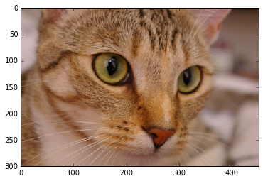
color_image = data.chelsea()

print(color_image.shape)
plt.imshow(color_image);

(300, 451, 3)

_config.yml

red_channel = color_image[:, :, 0]  # or color_image[..., 0]

Note: red_channel = color_image[all_the_rows, all_the_cols, 0thchannel]

plt.imshow(red_channel);

_config.yml

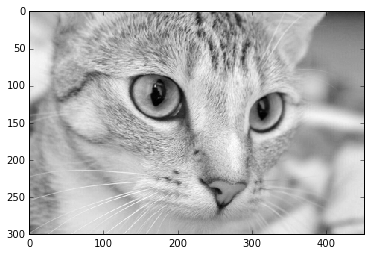
red_channel.shape

(300, 451)

from skimage import io
color_image = io.imread('../images/balloon.jpg')

import skdemo
red_image = np.zeros_like(color_image)
green_image = np.zeros_like(color_image)
blue_image = np.zeros_like(color_image)

red_image[:, :, 0] = color_image[:, :, 0] 
green_image[:, :, 1] = color_image[:, :, 1]
blue_image[:, :, 2] = color_image[:, :, 2]

skdemo.imshow_all(color_image, red_image, green_image, blue_image)

_config.yml

Note: np.zeros_like(color_image) Return an array of zeros with the same shape and type as a given array.

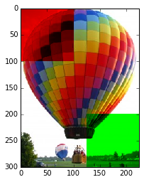
color_patches = color_image.copy()
# Remove green (1) & blue (2) from top-left corner.
color_patches[:100, :100, 1:] = 0
# Remove red (0) & blue (2) from bottom-right corner.
color_patches[-100:, -100:, (0, 2)] = 0
plt.imshow(color_patches);

_config.yml

from skimage import io
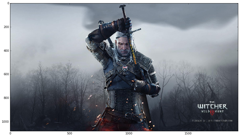
src = io.imread('/home/cobalt/Pictures/geralt.jpg') 
plt.figure(figsize = (16,8))
plt.imshow(src);

_config.yml

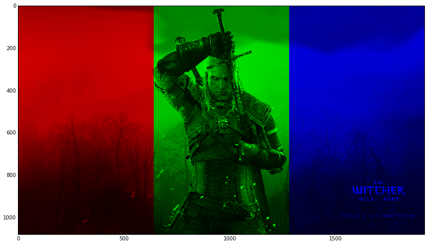
src_patches = src.copy()
col_by_3 = src_patches.shape[1]/3.
src_patches[:, :col_by_3, (1,2)] = 0
src_patches[:, col_by_3: 2*col_by_3, (0, 2)] = 0
src_patches[:, 2*col_by_3:, (0, 1)] = 0
plt.figure(figsize = (16,8))
plt.imshow(src_patches);

_config.yml

plt.figure(figsize = (16,8))

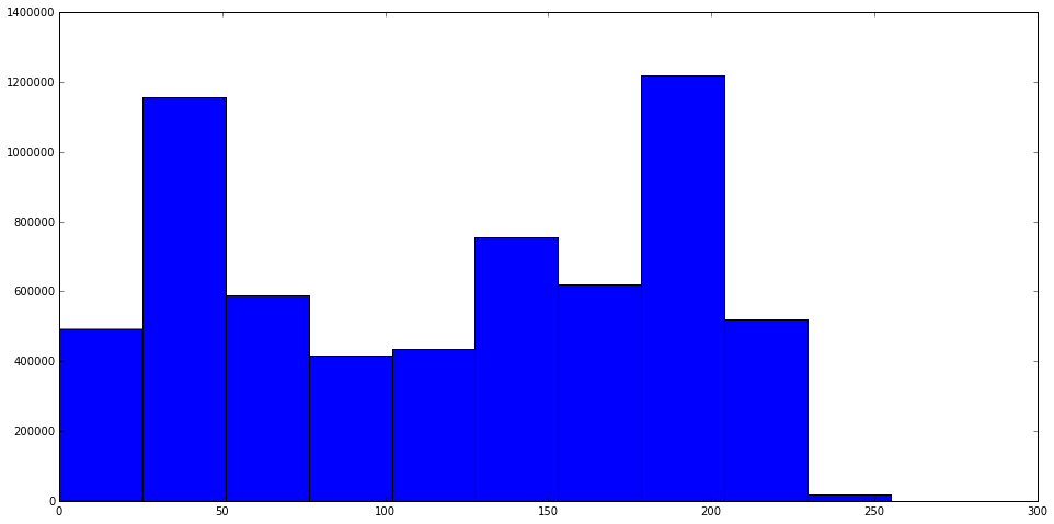
plt.hist(src.flatten())

(array([  491741.,  1156262.,   589345.,   415430.,   436289.,   755728.,
          619180.,  1219629.,   519156.,    18040.]),
 array([   0. ,   25.5,   51. ,   76.5,  102. ,  127.5,  153. ,  178.5,
         204. ,  229.5,  255. ]),
 <a list of 10 Patch objects>)

_config.yml

src.shape

(1080, 1920, 3)

np.rollaxis(src,axis=2).shape

(3, 1080, 1920)

for channel in np.rollaxis(src,axis=2):
    print(channel.shape)

(1080, 1920)
(1080, 1920)
(1080, 1920)

plt.figure(figsize = (16,8))

for channel in np.rollaxis(src,axis=2):
    plt.hist(channel.flatten())

_config.yml

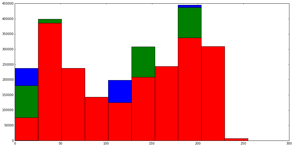
Note: Wrong order

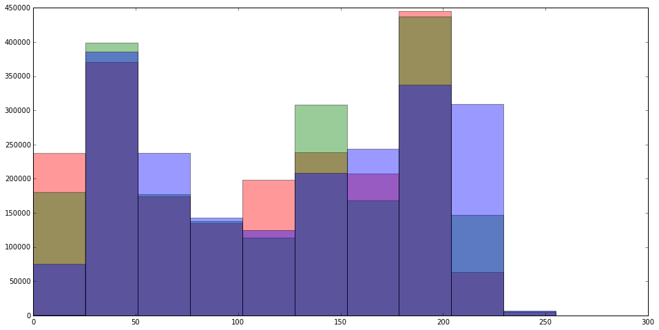
plt.figure(figsize = (16,8))

for color,channel in zip('rgb',np.rollaxis(src,axis=2)):
    plt.hist(channel.flatten(), color=color, alpha=0.4)

_config.yml

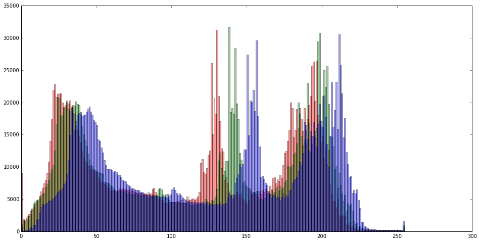
plt.figure(figsize = (16,8))

for color,channel in zip('rgb',np.rollaxis(src,axis=2)):    
    
    plt.hist(channel.flatten(), bins = 255, color=color, alpha=0.4)

_config.yml

from skimage import exposure

plt.figure(figsize = (16,8))

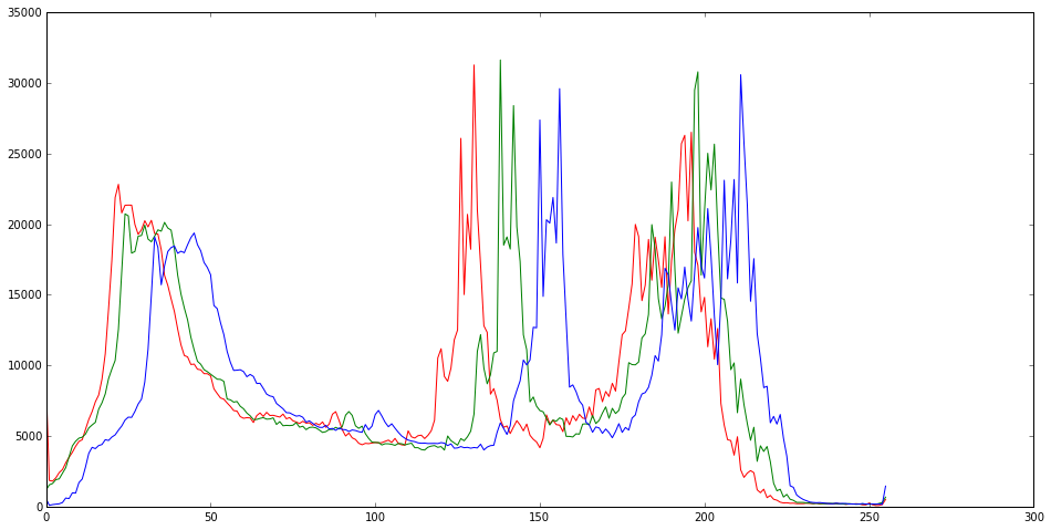
for color,channel in zip('rgb',np.rollaxis(src,axis=2)):
    freq, bin_centers = exposure.histogram(channel)
    plt.plot(bin_centers,freq, color=color);

_config.yml

from skimage import exposure

plt.figure(figsize = (16,8))

for color,channel in zip('rgb',np.rollaxis(src,axis=2)):
    freq, bin_centers = exposure.histogram(channel)
    plt.fill_between(bin_centers,freq, color=color, alpha=0.4);

_config.yml

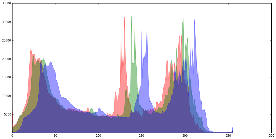
image = data.camera()
skdemo.imshow_with_histogram(image);

_config.yml

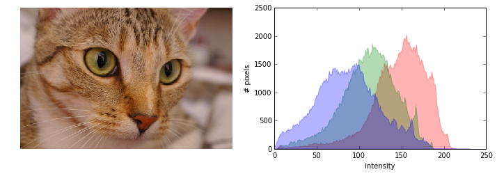
cat = data.chelsea()
skdemo.imshow_with_histogram(cat);

_config.yml

from skimage import io
src = io.imread('/home/cobalt/Pictures/geralt.jpg') 
skdemo.imshow_with_histogram(src);

_config.yml

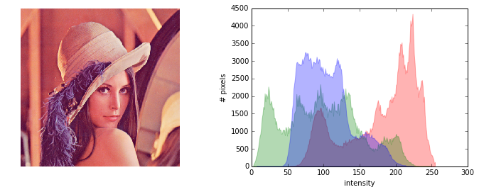
skdemo.imshow_with_histogram(data.lena());

_config.yml

from skimage import io
src2 = io.imread('/home/cobalt/Pictures/marian.jpg') 
skdemo.imshow_with_histogram(src2);

_config.yml

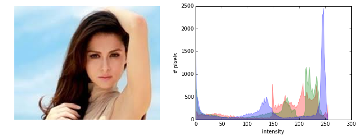
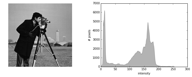
image = data.camera()
skdemo.imshow_with_histogram(image);

_config.yml

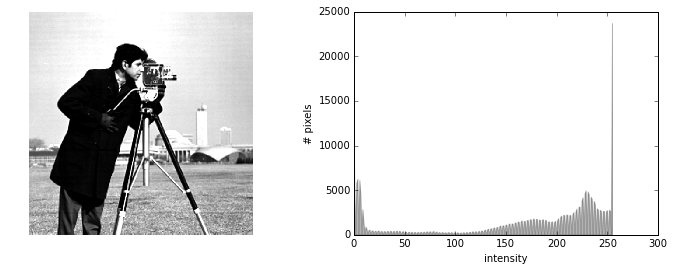
from skimage import exposure
high_contrast = exposure.rescale_intensity(image, in_range=(10, 180))
skdemo.imshow_with_histogram(high_contrast);

_config.yml

from skimage import exposure
high_contrast = exposure.rescale_intensity(image, in_range=(120, 180))
skdemo.imshow_with_histogram(high_contrast);

_config.yml

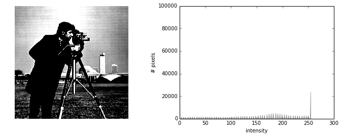
ax_image, ax_hist = skdemo.imshow_with_histogram(image)
skdemo.plot_cdf(image, ax=ax_hist.twinx())

_config.yml

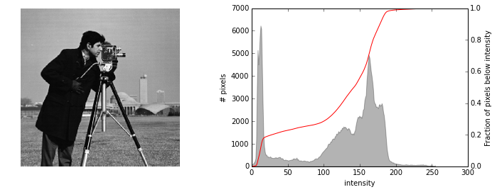
equalized = exposure.equalize_hist(image)


ax_image, ax_hist = skdemo.imshow_with_histogram(equalized)
skdemo.plot_cdf(equalized, ax=ax_hist.twinx())

_config.yml

equalized.dtype

dtype('float64')

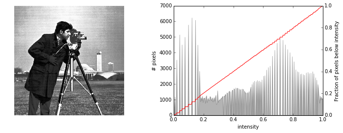
Unfortunately, histogram equalization tends to give an image whose contrast is artificially high. In addition, better enhancement can be achieved locally by looking at smaller patches of an image, rather than the whole image. In the image above, the contrast in the coat is much improved, but the contrast in the grass is somewhat reduced.

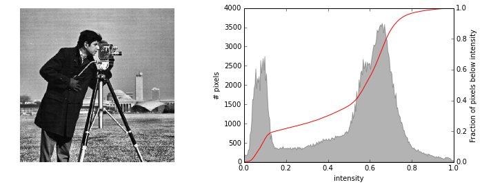
Contrast-limited adaptive histogram equalization (CLAHE) addresses these issues.

equalized = exposure.equalize_adapthist(image)


ax_image, ax_hist = skdemo.imshow_with_histogram(equalized)
skdemo.plot_cdf(equalized, ax=ax_hist.twinx())

_config.yml

equalized.dtype

dtype('float64')

exposure.equalize_adapthist?

An algorithm for local contrast enhancement, that uses histograms computed over different tile regions of the image. Local details can therefore be enhanced even in regions that are darker or lighter than most of the image.

skdemo.imshow_with_histogram(image);

_config.yml

threshold = 50
ax_image, ax_hist = skdemo.imshow_with_histogram(image)
ax_image.imshow(image > threshold)
ax_hist.axvline(threshold, color='red');

_config.yml

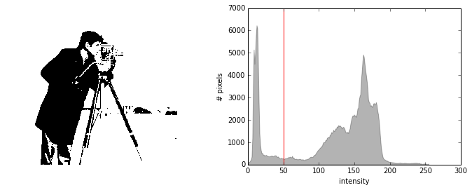
Note: the pants is not detected correctly.

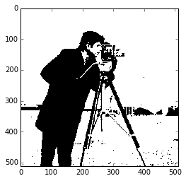
import skimage.filters as filters
threshold = filters.threshold_otsu(image)
print(threshold)

87

plt.imshow(image > threshold);

_config.yml

Reference:

[1] Juan Nunez Iglesias, Tony Yu, Image analysis in Python with scipy and scikit image 1 https://www.youtube.com/watch?v=MP-MTiCETYg
[2] http://scikit-image.org/ 

Written on April 3, 2015